MS Excel-Tips and Tricks and Notes
Thursday, June 25, 2015
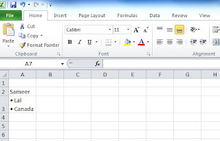
Create Bullet in MS Excel
To create the bullet character, press ALT+0149 (Press Alt and type
0149
on the numeric keypad and release Alt).
Friday, February 28, 2014
Our New Home: MS Excel
Please visit
MS Excel Advice
Link
http://msexceladvice.blogspot.ca/
That our new home.
Home
Subscribe to:
Posts (Atom)